绘制蛋白质谱差异表达分析后的火山图

张跃锋

################### author:zhangjian# updata:2023-1-8# version:1.0v# e-mail:zhangjian199567@outlook.com##################
目的

# 对蛋白质谱数据进行差异表达分析，并绘制其火山图
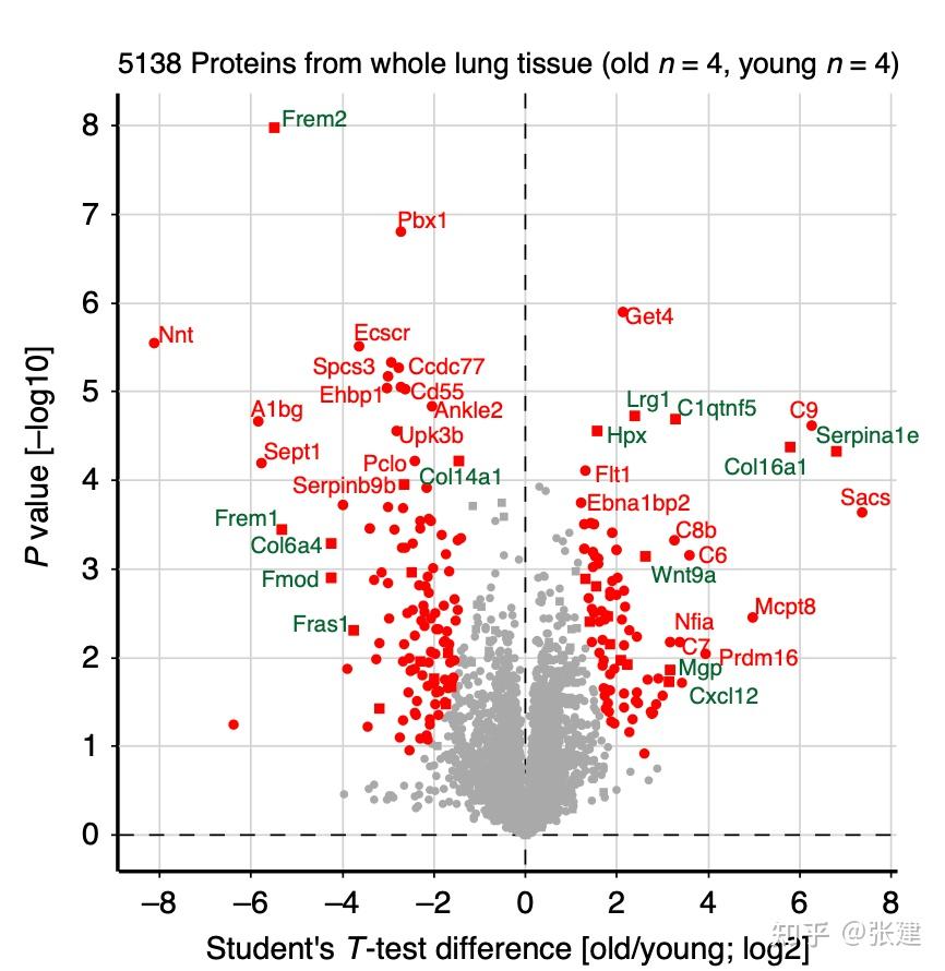
# 参考nature的绘图标准撰写相关代码
# 下图为nature的参考图形

使用到的软件

# 1蛋白质谱数据差异表达分析工具包
# 1.1 DEqMS
    DEqMS为蛋白质谱差异表达分析工具包（NOTE:不同的定量方法需要使用不同的参数）
# tips:蛋白质谱定量方法有:LFS,TMT,DIA

# 2.数据操作相关包
# 2.1 dplyr
       dplyr is primarily a set of functions designed to enable dataframe manipulation in an intuitive, user-friendly way
# tips:dplyr是一个很好用的数据框处理R package

# 2.2 matrixStats
    matrixStats为矩阵与数据框高效率处理工具

# 3.相关绘图R package
# 3.1 ggplot2
      ggplot2 鼎鼎大名的绘图工具包
# 3.2 ggthemes
      ggthemes 为ggplot2的主题包(下面的代码好像没有用到)
# 3.3 ggrepel
      ggrepel 超级好用的标注工具包

# 4.其他包
# 4.1 latex2exp
      latex2exp为一个TeX公式包，可以在ggplot2图中添加斜体、上下表、特殊的数学符号

# NOTE:如何安装相关工具包请自行google & baidu
# NOTE:想获得更多相关文档请自行搜索相关官方文档
代码

# NOTE: 下面的代码只适合LFS定量模式的蛋白质谱差异表达分析
# NOTE: 想对其他定量模式下获得的蛋白质谱数据进行差异表达分析，请自行查看DEqMS官方文档
# NOTE: 下面的代码主要是对蛋白质谱差异表达分析后的数据在火山图中对特定蛋白进行标注(注意上调与下调的蛋白进行了分开标注)
# This is a R scripts for draw volcano figure for MASS data of protein
# date:2023.1.9
# author:zahngjain
# e-mial:zhangjian199567@outlook.com

# PATH 1
# 1 install and loading package
# data analysis package
library(DEqMS)
library(matrixStats)
# draw figure package     
library(ggthemes)
library(ggplot2)
library(ggrepel)
library(latex2exp)
# data deal package
library(dplyr)

# 2 set analysis env
# 2.1 清除内存缓存
rm(list=ls())

# 2.2 set analysis folder
cat("当前的操作目录:",getwd())

# analysis env folder
# 可以自己进行替换
env_folder <- "/Users/zhangjian/Desktop/博士预/protein_mass_Volcanoplot"
setwd(env_folder)

# save folder
# 可以自己进行替换
save_folders <- "/Users/zhangjian/Desktop/博士预/protein_mass_Volcanoplot/output"

# data folder
# 可以自己进行替换
data_folders <- "/Users/zhangjian/Desktop/博士预/protein_mass_Volcanoplot/data"

# figure folder
# 可以自己进行替换
figure_folders <- "/Users/zhangjian/Desktop/博士预/protein_mass_Volcanoplot/figure"

# 2.3 loading protein mass data
mass_PSM <- read.csv(file.path(data_folders,
                               "deal_20221107_WPP_LFQ_Nor_proteins.csv"))
# head(mass_PSM)

# 2.4 提取gene ID
mass_PSM_ref <- mass_PSM[,c(3,4)]
colnames(mass_PSM_ref) <- c("gene","lable")
# head(mass_PSM_ref)
# NOTE:蛋白组质谱分析(LS-MS) -> 搜库(分析公司的任务)获得的蛋白质谱文件包含搜索到的多肽属于哪一个蛋白和gene

# PATH 2 DEqMS 差异表达分析
# 1 extract protein dataframe
# 1.1 set protein dataframe col index
extract_columns = seq(25,30)  

# head(mass_PSM[,TMT_columns])
# 选择25-30列，也就是所有的COUNT数据
# NOTE:这个不同的数据提取，不同的数据有不同的设置

# 1.2 filter at 1% protein FDR and
# 筛选 q.value(FDR) 值小于0.01的搜库结果
filter_mass_PSM <- mass_PSM[mass_PSM$Exp..q.value..Combined<0.01,extract_columns]   

# 通过过滤的蛋白比例
ratio <- length(rownames(filter_mass_PSM))/length(rownames(mass_PSM))
print(ratio)

# 1.3 filter_mass_PSM 矩阵行名设置
rownames(filter_mass_PSM) <- mass_PSM[mass_PSM$Exp..q.value..Combined<0.01,]$Accession
write.csv(filter_mass_PSM,file.path(save_folders, "mass_PSM_frame_FDR_0.01_9244-NC.csv"))

# 1.4 protein dataframe structure
# The protein dataframe is a typical protein expression matrix structure
# Samples are in columns, proteins are in rows
# use unique protein IDs for rownames
# to view the whole data frame, use the command View(filter_mass_PSM)
# View(filter_mass_PSM)

# 2. data deal
# If the protein table is relative abundance (ratios) or intensity values, Log2 transform the data.
# Systematic effects and variance components are usually assumed to be additive on log scale (Oberg AL. et al JPR 2008; Hill EG. et al JPR 2008).
# 如果蛋白数据为相对丰度或者

filter_mass_PSM.log = log2(filter_mass_PSM+1)         #数据取对数
filter_mass_PSM.log = na.omit(filter_mass_PSM.log)    #remove rows with NAs
# View(dat.log)
boxplot(filter_mass_PSM.log,las=2,main="20221107_WPP_LFQ_Nor_proteins")   
# Use boxplot to check if the samples have medians centered. if not, do median centering.

# Here the data is already median centered, we skip the following step.
# 由于数据表达量足够一致，所以可以不进行标准化
# dat.log = equalMedianNormalization(dat.log)

# 3 set group factor infor
# if there is only one factor, such as treatment. You can define a vector with
# the treatment group in the same order as samples in the protein table.
cond = as.factor(c("sample_9244","sample_9244","sample_9244","NC","NC","NC"))

# The function model.matrix is used to generate the design matrix
design = model.matrix(~0+cond) # 0 means no intercept for the linear model
# 这里是设计一个对比矩阵，其做法原理可以详见：https://treeh.cn/?id=21

colnames(design) = gsub("cond","",colnames(design))    #去除表格中的cond字符
# View(design)

# 4.set contrast infor
# you can define one or multiple contrasts here
# 设计哪些组间需要对比
x <- c("sample_9244-NC")
contrast =  makeContrasts(contrasts=x,levels=design)    #按照x的对比方式，对design的样本分组对样本进行比较
#View(contrast)

# 5. build Linear Model and
# 线性拟合模型构建
fit1 <- lmFit(filter_mass_PSM.log,
              design)
# Compute Contrasts from Linear Model Fit
fit2 <- contrasts.fit(fit1,
                      contrasts = contrast)
# Given a linear model fit to microarray data, compute estimated coefficients and standard errors for a given set of contrasts.
# Empirical Bayes Statistics for Differential Expression
fit3 <- eBayes(fit2)
# Given a linear model fit from lmFit, compute moderated t-statistics, moderated F-statistic, and log-odds of differential expression by empirical Bayes moderation of the standard errors towards a global value.
# 具体介绍参考自help(contrasts.fit)、help(eBayes)
# assign a extra variable `count` to fit3 object, telling how many PSMs are quantifed for each protein
# count_columns = seq(9)#选择16-34列中、间隔1列的数据，也就是所有的PSMs数据
psm.count.table = data.frame(count = rowMins(as.matrix(mass_PSM[,9])), row.names =  mass_PSM$Accession)
# rowMins: Calculates the minimum for each row (column) of a matrix-like object
fit3$count = psm.count.table[rownames(fit3$coefficients),"count"]#数据导入fit3中
fit4 = spectraCounteBayes(fit3)
# Peptide/Spectra Count Based Empirical Bayes Statistics for Differential Expression. This function is to calculate peptide/PSM count adjusted t-statistics, p-values.
head(psm.count.table)


# 提取第一个对比组
DEqMS.results = outputResult(fit4,coef_col = 1)  # sample_9244-NC group
# 提取其他对比组(如果有多个的前提下)
# DEqMS.results = outputResult(fit4,coef_col = 2)
# a quick look on the DEqMS results table
# 快速查看蛋白质谱差异表达结果
head(DEqMS.results)
# Save it into a tabular text file
write.csv(DEqMS.results,file.path(save_folders, "DEqMS.results.sample_9244-NC.csv"))

# PATH 3 结果可视化
# 火山图（所有基因）
# 1. 数据处理
# 1.1 添加-log10信息
Volcano_input_data <- as.data.frame(DEqMS.results)
rownames(Volcano_input_data) <- Volcano_input_data$gene
Volcano_input_data <- merge(Volcano_input_data,mass_PSM_ref,by="gene",sort=FALSE)
head(Volcano_input_data)
Volcano_input_data$"-log10(adj.P.Val)" <- -log10(Volcano_input_data$adj.P.Val)

# 1.2 添加分组信息
Volcano_input_data$Group <- "not"
Volcano_input_data$Group[which((Volcano_input_data$adj.P.Val < 0.05) & (Volcano_input_data$logFC > 0.5))] = "up"
Volcano_input_data$Group[which((Volcano_input_data$adj.P.Val < 0.05) & (Volcano_input_data$logFC < -0.5))] = "down"
table(Volcano_input_data$Group)       #统计分组信息
# 同时在这里要注意的一点是这个logFC的cutoff一般就是设置为1，但是如果到筛选出的基因过多就要将cutoff阈值进行一个提高一下看看。

# 1.3 搜索差异表达前50个protein进行标记
# Volcano_input_data$label_1 = NA
# Volcano_input_data <- Volcano_input_data[order(Volcano_input_data$adj.P.Val),]
# up.genes <- head(Volcano_input_data$lable[which(Volcano_input_data$Group == "up")],50)
# down.genes <- head(Volcano_input_data$lable[which(Volcano_input_data$Group == "down")],50)
# Volcano_input_data$label[match(Volcano_input_data.top.genes,Volcano_input_data$lable)] <- Volcano_input_data.top.genes
# table(Volcano_input_data$label)

# 1.4 标记自己提供的蛋白名称
# 使用自己提供的蛋白名称进行数据框
down <- as.data.frame(c("Cmc2","Ndufa4","Cox5b","Cox6a1","Mtco2","Mtco1","Cox7a2","Cox7b2","Cox6c","Cox4i1"))
colnames(down) <- "lable"
down_Volcano_input_data_lable <- left_join(down,Volcano_input_data,by="lable")
write.csv(down_Volcano_input_data_lable,file.path(save_folders, "down_Volcano_input_data.csv"))
head(down_Volcano_input_data_lable)

up <- as.data.frame(c("Tnip1","Gdf15","Rab2a"))
colnames(up) <- "lable"
up_Volcano_input_data_lable <- left_join(up,Volcano_input_data,by="lable")
write.csv(up_Volcano_input_data_lable,file.path(save_folders, "up_Volcano_input_data.csv"))
head(up_Volcano_input_data_lable)

# 1.4 draw Volcano
# 使用ggpolt 进行绘图
p <- ggplot(Volcano_input_data,
            aes(x = logFC,
                y = -log10(adj.P.Val),
                colour=Group)) +  
      # 绘制点图(point figure)
      geom_point(alpha=0.5,
                 size=2) +
      # point点颜色设置
      scale_color_manual(values=c("#546de5",
                                  "#798a9c",
                                  "#ff4757"))+
      # 在figure中添加水平线
      geom_vline(xintercept=0,
                 lty=4,
                 col="black",
                 lwd=0.3) +  
      # 在figure中添加垂直线
      geom_hline(yintercept = 0,
                 lty=4,
                 col="black",
                 lwd=0.3) +  
      # figure 标题设置
      labs(x="Fold Change (log2)",
           y= TeX(r"(\textit{P} value (-log10) )"),
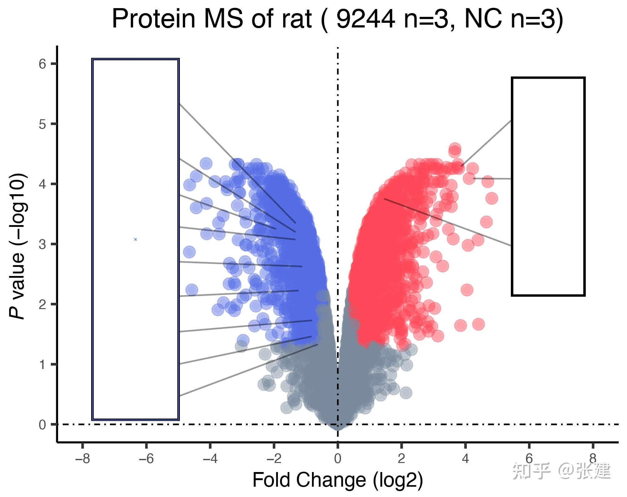
           title="Protein MS of rat ( 9244 n=3, NC n=3)") +
      # figure 中给点添加名称(down)
      geom_text_repel(data=down_Volcano_input_data_lable,
                      aes(logFC,
                          -log10(adj.P.Val),
                          label= lable,
                          colour=Group),
                      fontface="bold" ,
                      size = 1.8,
                      segment.alpha = 0.4,
                      segment.size = 0.3,
                      segment.color = "black",
                      box.padding=unit(1, "lines"),
                      point.padding=unit(0.1, "lines"),
                      force = 1,
                      max.iter = 3e3,
                      xlim=c(-8, -5),
                      ) +
       # figure 中给点添加名称(up)
       geom_text_repel(data=up_Volcano_input_data_lable,
                       aes(logFC,
                           -log10(adj.P.Val),
                           label= lable,
                           colour=Group),
                       fontface="bold" ,
                       size = 1.8,
                       segment.alpha = 0.4,
                       segment.size = 0.3,
                       segment.color = "black",
                       box.padding=unit(1, "lines"),
                       point.padding=unit(0.1, "lines"),
                       force = 1,
                       max.iter = 3e3,
                       xlim=c(5, 8),) +
      # figure 中图例设置
      guides(color=guide_legend(override.aes = list(size=10)),) +
      # figure x轴坐标范围与刻度设置
      scale_x_continuous(limits=c(-8,8),
                         breaks=seq(-8,8,2)) +
      # figure y轴坐标范围与刻度设置
      scale_y_continuous(limits=c(0,6),
                         breaks=seq(0,6,1)) +
      # figure 加载默认主题
      theme_classic()+
      # figure 定制主题
      theme(plot.title = element_text(hjust = 0.5),    # 图片标题居中
            legend.position="none",                    # 不显示图例
            legend.title=element_text(size = 10,
                                      face = "normal",
                                      family="Times"), # 图片名称设置(大小，字体)
            text = element_text(size = 10,
                                family="sans"),        # 所有文本的基础设置
            title = element_text(size = 10),           # 所有标题的基础设置
            axis.title.x = element_text(size = 9),    # X坐标轴名称设置
            axis.title.y = element_text(size = 9),    # Y坐标轴名称设置
            axis.text.x = element_text(size = 6),     # X坐标轴刻度设置
            axis.text.y = element_text(size = 6),     # Y坐标轴刻度设置
            axis.line.x=element_line(linetype=1,
                                     color="black",
                                     size=0.4),        # X轴线宽与颜色
            axis.line.y=element_line(linetype=1,
                                     color="black",  
                                     size=0.4))        # Y轴值线宽与颜色

# 1.5 draw Volcano
# 使用ggsave保存绘图
ggsave(file.path(figure_folders,
                 "DEqMS.results.sample_9244-NC.pdf"),
       plot = last_plot(),
       width = 10,
       height = 8,
       units = "cm")结果

# 下面的为此代码绘制的火山图
# 可能也不是很完美，如有相关建议请联系本人的邮箱
# 禁止转载
# 由于相关原因，图片部分隐藏